University of Notre Dame
Aerospace and Mechanical Engineering

AME 654: Geometric Nonlinear Control
Final Exam

B. Goodwine
Fall, 2003
Issued: December 15, 2003
Due: December 20, 2003

  1. This problem will consider feedback linearization of the shimmying wheel problem.

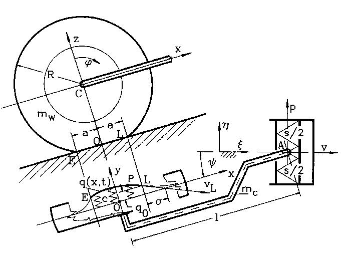
    If we assume that the tire is rigid, i.e., q(x,t) = 0 and that it rolls without slipping, the equations of motion are


      \begin{eqnarray*}\ddot{\theta} &=& \frac{ - \frac{v}{l} \left( \mbox{sec}^2 \the...
	    ...ec } \theta \left( v +
	    l \dot \theta \sin \theta \right) }{r}.
	    \end{eqnarray*}


    1. Follow the procedure outlined in class to find an output function which makes this system feedback linearizable. Since the wheel rotation angle is cyclic, we can ignore the third equation, and full state linearization requires a relative degree of three.
    2. Simulate the system (both controlled and uncontrolled) using the following parameter values: mc = 1.5kg, mw = 2.75kg, l = 0.152 m, r = 0.1m, k = 75N/m and v = 1m/s.
  2. Sastry, 3.27.
  3. Investigate the bifurcations of equilibria for the system

    \begin{displaymath}\dot x = f(x,\mu) \end{displaymath}

    near $\mu = 0$ with:
    1. $f(x,\mu) = \mu - x^2$
    2. $f(x,\mu) = \mu x - x^2$
    3. $f(x,\mu) = \mu^2 x - x^3$
    4. $f(x,\mu) = \mu + x^3$
    5. $f(x,\mu) = \mu^2 \alpha x + 2 \mu x^3 - x^5$ for various $\alpha$.
    In each case onstruct the bifurcation diagram.


I suppose it is possible that the stereotype of the wicked scientist dissuades some youngsters from entering the profession, but the world today is so topsy-turvy that perhaps as many are attracted as are repelled by the prospect of a career of malefaction.

--- Sir Peter Medawar, Advice to a Young Scientist.


Last updated: December 15, 2003.
B. Goodwine (jgoodwin@nd.edu)