Bill Goodwine's Courses

Consider the system illustrated in Figure 7.9 in the course text. Assume there are 6 masses each with a mass of 2 and each of the 7 springs has a spring constant of 3 (ignore the spring constants indicated in the figure).

1. Determine the equations of motion for the system.
2. Write a FORTRAN, C or C++ program to determine an approximate numerical solution for the system assuming all the initial conditions are zero except the initial velocity of the 6th mass is -2 and f(t)=0. You may use Euler's method or RK. Plot the solution in a manner that clearly communicates the nature of the solution (is there a wave traveling down the chain?).
3. Verify your answer to the previous problem using ode45() in Matlab.
4. Use the Matlab place() function to determine the values of the ks that place the eigenvalues for the system under full state feedback (that means f = k1 x1 + k2 x2 + ... k20 x20) at -1, -1.1, -1.2, ..., -2.1. Modify your program to include the force and plot the solution.
5. Use the Matlab place() function to determine the values of the ks that place the eigenvalues for the system under full state feedback at -1, -1.1, -1.2, ..., -1.9 and -.1 + i, -.1 - i. Modify your program and plot the solution and compare it to the solution in the previous part and explain any differences and whether or not the differences are what you would expect.
6. Use the matlab lqr() command to make the motion of the 4th mass become small much faster than the other masses. Modify your program and plot the solution.

Notes for part 6:

• I downloaded building.m and buildingrhs.m
• I changed the initial conditions in building.m to be [10 10 10 10 10 10 10 10 10 10] and also edited to only plot once.
• Then I ran:

  Code: Select all

  >> Q = eye(10);
  >> lqr(A,B,Q,[1])
  
  ans =
  
      0.1488    0.1888   -0.4697    0.7217    0.7565    0.5678   -2.0227    1.4118    2.6190    2.4976
  

  I copied the gains in ans into the K matrix in buildingrhs.m and then ran building.m again (I edited it to only plot once) and got the following plot.
  
• Then I ran

  Code: Select all

  Q(5,5) = 100
  
  Q =
  
       1     0     0     0     0     0     0     0     0     0
       0     1     0     0     0     0     0     0     0     0
       0     0     1     0     0     0     0     0     0     0
       0     0     0     1     0     0     0     0     0     0
       0     0     0     0   100     0     0     0     0     0
       0     0     0     0     0     1     0     0     0     0
       0     0     0     0     0     0     1     0     0     0
       0     0     0     0     0     0     0     1     0     0
       0     0     0     0     0     0     0     0     1     0
       0     0     0     0     0     0     0     0     0     1
  
  >> lqr(A,B,Q,[1])
  
  ans =
  
      2.9803    2.8564   -0.2577    6.2080   -0.6458    3.7663   -1.3699    7.5652    6.9451    3.8588
  

  and copied those gains into buildingrhs.m and re-ran building and got the following plot.
  
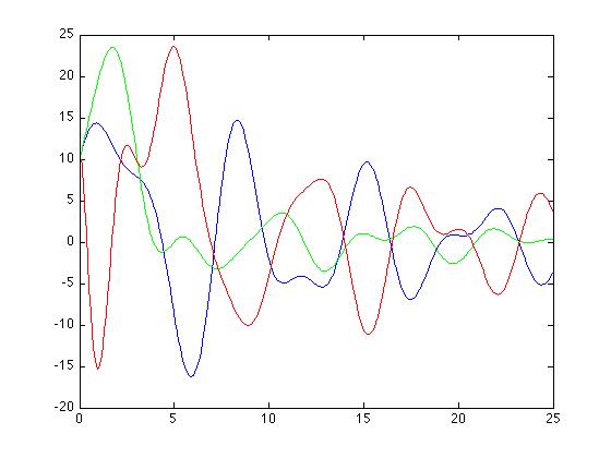
  You can observe that the green curve is smaller relative to the red and blue curves, which reflects a higher weighting for that element.

Prof. Goodwine,
For part 4, Matlab is unable to perform the "place" command. It says either (A,B) is nearly uncontrollable or the specified locations are too close to each other. I'm not sure why the specified locations would be wrong. I played around with them some, but to no avail.

kroshak wrote:Prof. Goodwine,
For part 4, Matlab is unable to perform the "place" command. It says either (A,B) is nearly uncontrollable or the specified locations are too close to each other. I'm not sure why the specified locations would be wrong. I played around with them some, but to no avail.

The TA is working on that right now. If we can't find a solution I'll scale it back to the size of the problem I did above and it will work. I'm sorry to delay your homework but you'll just have to hang out a while. If you want to fiddle with it some more, then I'd recommend trying to space out the eigenvalues more, i.e., have them .2 apart, or .5 apart, etc. If that doesn't work, then there probably are just too many masses for it to work effectively.

Are we still responsible for turning in problems 5 and 6 from last week's handout with this week's homework?

sbonomo wrote:Are we still responsible for turning in problems 5 and 6 from last week's handout with this week's homework?

No, that's going to be on next week's homework. So, if you want to work ahead, do them, but they won't be due until next Wednesday.

For parts 3,4, and 6, do we just provide the plot or should we provide our code as well?

jdeoreo wrote:For parts 3,4, and 6, do we just provide the plot or should we provide our code as well?

Submit the code for part 4 too. The purpose of the problem is to show that you know how to put the force into the FORTRAN program. You can leave the program out for the other two though.

Can a solution with only real eigenvalues exhibit oscillatory behavior? For the pole placement problem with only real negative eigenvalues, the solutions I got exhibited oscillating. Even though the solutions are composed of linear combinations of real exponentials, this is possible if the coefficients and the exponential terms are arranged in a special way, right? However, unlike a sinusoid which oscillates forever, the number of oscillations of a linear combo of exponentials is limited by the number of exponentials in the combination (for example, if three exponentials, maximum of 2 peaks) right?
Thank you.

mkiener wrote:Can a solution with only real eigenvalues exhibit oscillatory behavior? For the pole placement problem with only real negative eigenvalues, the solutions I got exhibited oscillating. Even though the solutions are composed of linear combinations of real exponentials, this is possible if the coefficients and the exponential terms are arranged in a special way, right? However, unlike a sinusoid which oscillates forever, the number of oscillations of a linear combo of exponentials is limited by the number of exponentials in the combination (for example, if three exponentials, maximum of 2 peaks) right?
Thank you.

I believe that is correct -- one less peak than the number of exponentials is possible.