Homework 3, due 15 September 2005.
Posted: Fri Sep 09, 2005 6:46 am
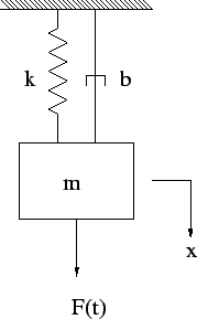
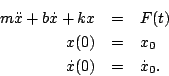
We love the system illustrated in the following figure so much that we are going to solve every reasonable permutation of it. The reason we love it so much is, of course, that it is so broadly applicable to many important engineering problems that entire text books are devoted to it.
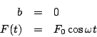
- For the case where
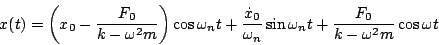
- Determine the solution in the case where
- Plot the solution. A hand sketch is adequate as long as it is qualitatively accurate.
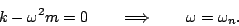
- When the forcing frequency is very close, but not exactly equal, to the natural frequency which solution (the solution you just determined or the one from class) is correct? Plot the solution. Again, a hand sketch is adequate as long as it is qualitatively accurate.
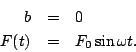
- Determine the solution when
- Assume for this problem that there is gravity.
- Derive the equations of motion when x is measured from the unstretched position of the spring.
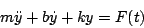
- Show that the equation of motion for the system is
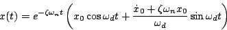
- For damped unforced (F(t)=0) oscillations, we showed in class that the (homogeneous) solution to the equation given at the top of the page is
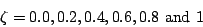
- Determine the (homogeneous) solution when
- Determine the (homogeneous) solution when
- For the damped unforced oscillation case where