Bill Goodwine's Courses

Unless otherwise indicated, each problem that requires you to write a computer program must be done in C, C++, FORTRAN or another language explicitly approved by the instructor.

1. Complete any of the problems that you skipped from Homework 4.
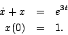
2. Determine an approximate numerical solution to
   • 
   using Euler's method and 4th order R-K. Then cut the time step in half. Does the local truncation error after the first time step behave as expected? Does the global accumulated error behave as expected?
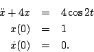
3. Consider
   • 
   This is an example of undamped forced vibrations where the forcing frequency and the natural frequency are the same. Here m=1, k=4, F=4 and the forcing frequency is 2.
   1. Determine the analytical solution.
   2. Convert this second order equation into two first order equations.
   3. Write a computer program that uses Euler's method to compute an approximate solution for the time interval t=0 to t=10. Determine a good time step by comparing the approximate solution to the analytical solution.
4. How to use Matlab.
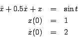
   Matlab has a built-in function called ode45() that is an implementation of the 4th order R-K method. As an example of how to use it, let's use it to numerically solve
   • 
   which is equivalent to the two first order equations
   • 
   To use ode45() you must create a new Matlab function. The easiest way to make a new function is to make a *.m file where the * is the the new function name.
   
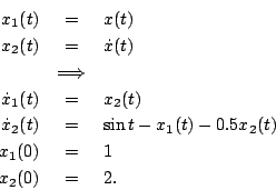
   Since we like to solve differential equations with f(x,t) in the equation, let's created a new function called f that needs an x and t as arguments. In this example, the following would go inside the file called "f.m" and the file f.m should be in the same directory in which you started Matlab:

   Code: Select all

   function xdot = f(t,x)
    xdot = zeros(2,1);
    xdot(1) = x(2);
    xdot(2) = sin(t) - x(1) - 0.5*x(2);
   

   Note that the order in the first line, f(t,x) is important. You'll get the wrong answer with f(x,t) there. Now, to compute the solution, simply type the follwing at the Matlab prompt:

   Code: Select all

   >> [t,x] = ode45(@f,[0 10],[1 2])

   This will give back a vector of times and a matrix for x. The first column of x will be x(1) and the second column will be x(2). The [0,10] is the time interval (t=0 to t=10) and the [1 2] are the initial conditions. To plot the answer, just type

   Code: Select all

   >> plot(t,x(:,1))

   Note: if you want to call your function something other than f you have to change f in three places: the first line of the file f.m, the name of the file and the first argument of ode45().
   1. Reproduce the above steps to use ode45() to determine an approximate solution to the equation for problem 3. Fixed Monday morning. This incorrectly referred to problem 2.
   2. Use ode45() to compute a numerical approximation to the solution in problem 2 and compare it with your answer. Fixed as well.
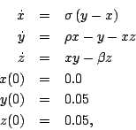
5. Consider the famous Lorenz equations
   • 
   where
   • 
   1. Using 4th order Runge-Kutta determine an approximate numerical solution to these equations for the time range t=0 to t=50. Submit a 3D plot of (x,y,z). Be sure to experiment with the time step to ensure that your solution is accurate. The Matlab plot3() function will probably be useful. A quick google search will probably give you an idea of what the plot should look like.
      
      Hint: for one first order equation, 4th order R-K uses w1, w2, w3 and w4. To do this for three equations, you will need something like w1, w2, w3, w4, v1, v2, v3, v4, u1, u2, u3 and u4, where the w's are for the first equation, the v's are for the second and the u's are for the third.
   2. Use Matlab's ode45() to compute an approximate solution and plot the result.
   3. (5 points extra credit) Explain the significance of these equations.
6. Consider the rather innocent-looking differential equation
   • 
   1. Show that
      • 
      is the solution to the differential equation.
   2. Write a computer program to determine an approximate solution using Euler's method to this first order differential equation.
   3. Submit a plot of the approximate solution and the exact solution for this equation for the time interval from t=-1 to t=1. Use trial and error to determine an appropriate step size by comparing your approximate numerical solution to the exact solution for different step sizes and ensure that the magnitude of the maximum error is less than 0.001. Hint the step size has to be pretty small! Be sure to submit your code as well.
   4. Use the Matlab ode45() function to solve the equation. Submit your code and a plot of the solution and the exact solution. Does Matlab give the correct answer?
   5. (5 points extra credit) Figure out how to tweak the tolerances in ode45(). Is it possible to get an accurate solution?
   6. Write a matlab script to implement the same method you used for part (b) above. An example script using Euler's method to solve the equation
      • 
      would look like the following:

      Code: Select all

      >> x(1) = -6;
      >> dt = 0.01;
      >> t = 0:dt:10;
      >> for i=2:length(t)
      x(i)=x(i-1)+sin(t(i-1))*dt;
      end
      >> plot(t,x)
      

      If you had to use the same size time step as you determined was necessary in part (c), determine approximately how long it will take for Matlab to solve it in this manner.