Bill Goodwine's Courses

Posted: **Wed Apr 04, 2007 11:59 am**

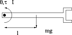
Consider the robot arm illustrated in the following figure (the same as we did in class).
Write a computer program using 4th order R-K to determine an approximate solution to this system when controlled by PID control (the equations were given in class). This program should determine a solution to the original, nonlinear equations. The point of the next problem is to show that the conclusions we make for the linearized equations hold for the nonlinear equations, at least for values of the angle where the approximation is valid.
Using this program, verify the following "rules of thumb" for PID control using the definitions of ise time, peak time, overshoot, settling time and steady state error from the following figure. Be sure to submit your program and graphs to support your demonstration that the rules are correct.
1. For proportional control, i.e., kp > 0, kd = 0 and kI=0, the solutions are oscillatory, and increasing kp increases the frequency of oscillation (which decreases the rise time and peak time) but decreases the mean steady state error. The settling time is infinite. Hint pick a starting value of kp=5.
2. If derivative control is added to the proportional controller, i.e., kp > 0, kd > 0 and kI=0, then
  - for small kd the solutions are decaying oscillations;
  - increasing kd decreases the settling time;
  - increasing kd sufficiently eliminates the oscillatory behavior completely, resulting in an solution which exponentially decays to the final, steady state value;
  - increasing kp decreases the final steady state error;
  - increasing kp decreases the rise time.
  Hint pick a starting value of about kd=0.5.
3. Adding integral control (PID control)
  - eliminates the steady state error, even for small values of kp,
  - increasing kI generally increases the overshoot and settling time;
  - increasing kp decreases rise time, but may increase overshoot;
  - increasing kd increases damping and stability.
  Hint: pick a starting value of about kI=0.5.
Determine the region in the complex plane where the poles for a second order system should be located so that
1. the maximum overshoot is less than 5%
2. the 1% settling time is less than 4 seconds
3. both of the above.
At this point we have a good grip on second order systems. Unfortunately, the world isn't entirely composed of second order systems. In order to apply what we know to second order systems, it will be useful to determine the approximate effect of poles and zeros in addition to a complex conjugate pair for a second order system. Most, but not all of this problem will be done using matlab.
1. Effect of additional poles far to the left. Consider
  Plot the step response using Matlab. Plot the step response of a system with G(s) having another pole far to the left, say at s=-10. Are the responses comparable?
2. Add a zero to G(s) far to the left. What is the effect on the step response?
3. Add a zero to G(s) in the left half plane relatively close to the imaginary axis. What is the effect on the step response?
4. Add a zero to G(s) in the right half plane relatively close to the imaginary axis. What is the effect on the step response?
5. Add a pole to G(s) in the left half plane relatively close to the imaginary axis. What is the effect on the step response?
6. Without computing or plotting anything, what will be the effect of adding a pole to G(s) near the imaginary axis near the imaginary axis in the right half plane?
7. Add a zero to G(s) at s=-1 and a pole to G(s) at s=-0.95. What is the effect on the step response? What can you say in general about a pole and zero that are close together?
Extra credit. Do the partial fraction expansion for the step response of the second order system, G(s) in the previous problem. Also do the partial fraction expansion for the second order system with an added zero (hint: put 1/r*(s+r) in the numerator). Based on these, prove your conclusions from the previous problem by considering the cases when r is positive and large, positive and small and negative and small.
Match the plots of the location of the poles and zeros of a transfer function with the plots of the unit step response. In each case, justify your answer.
Pole-zero maps
Step responses

Bill Goodwine's Courses

Homework 8 with links to images.

Homework 8 with links to images.