Bill Goodwine's Courses

Update Friday, April 20, 14:45. Two extra credit problems added.

1. If
   • 
   and
   • 
   prove the multiplication rule for complex numbers in polar form, i.e., that the angles add and the magnitudes multiply so that
   • 
2. In class we determined regions in the complex plane where the poles of a second order system will meet overshoot and settling time requirements. The rise time specification is a bit harder to nail down. Rather than delve into it analytically, this problem will let you verify that one approximation via a few numerical experiments.
   
   A common approximation is to use
   • 
   1. Pick three different sets of complex conjugate pairs of poles (with different damping ratios and different natural frequencies) and use the matlab step() function to verify that this is at least an o.k approximation. Also verify that the settling time and overshoot are what would be expected based upon the second order pole locations.
   2. Plot the region in the complex plane where a pair of second order complex conjugate poles should be located so that the rise time is less than 2 seconds.
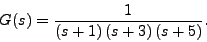
3. Consider
   • 
   1. Sketch the root locus for this transfer function.
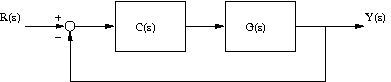
   2. In the following block diagram if C(s)=k, based upon your root locus plot, describe what will happen as k gets large to the percentage overshoot of the response, y(t), if the input, r(t) is a step input.
      • 
   3. Using your root locus plot, determine a k value so that the percentage overshoot is approximately 20%. Verify it using the matlab step() command.
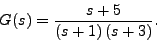
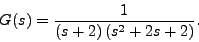
4. Consider
   • 
   1. Sketch the root locus plot for this transfer function.
   2. Based upon your root locus plot, describe what will happen to the step response of this transfer function if it is placed in the same block diagram as above as k gets large. Specifically describe what will happen to the percentage overshoot, the settling time and the rise time.
5. Sketch the root locus plot for
   • 
   As k gets large, what can you say about the stability of the step response of this system under unity feedback (the same block diagram as above)?
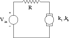
6. Consider a dc motor driven by a circuit as illustrated in the following figure. Assume that the shaft of the motor has a moment of inertia J.
   • 
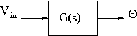
   1. If the following block diagram represents this system, determine G(s).
      • 
   2. Referring to the block diagram in the second problem above (with a C(s) and G(s)), determine the transfer function from the desired angular position to the actual angular position for the cases of
      • proportional control;
      • proportional plus derivative control;
      • proportional plus derivative plus integral control; and
      • proportional plus integral control.
   3. Without substituting anything for C(s) or G(s) determine the transfer function from the desired angle to the actual angle.
   4. For each of the control methods in part c, if you were to sketch the root locus plot to determine how the poles of the transfer function varied as k went from 0 to +infinity, what would be the transfer function that you would use? In other words, the rules to plot the root locus are described in terms of a particular transfer function that is not the "overall" transfer function (e.g., on the real axis, the root locus is to the left of an odd number of poles plus zeros of the transfer function).
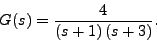
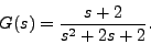
7. Sketch the root locus for
   • 
8. Finally, for the transfer function in the previous problem, determine G(s) where s=1+i by
   1. substituting s into G and evaluating it; and,
   2. measuring the angle and distance from each of the poles and zeros of G(s) and computing the magnitude and angle of G(s) based upon those measurements.
9. (Extra credit) Sketch the root locus plot for
   • 
10. (Extra credit) Sketch the root locus plot for
    • 

Could you explain the distinction between Prob. 3 and Prob. 4? Thanks

awulz wrote:Could you explain the distinction between Prob. 3 and Prob. 4? Thanks

The equations somehow got messed up (they were supposed to be different), so there basically isn't much distinction.

6b:
I solved the proportional control case in two different ways and got two different answers, so I am hoping you can show me what I'm doing wrong. The first way was using a block diagram, where the new transfer function should work out to be k_p*G(s) / (1+k_p*G(s)), where G(s) is the transfer function from part a. The second way is going back to the initial circuit and substituting k_p*(theta_d-theta) for tau (torque); for part a, I had tau = J*(d^2/dt^2(theta))... so that's the substitution.
The answer from using the block diagram made sense, but using the tau substitution on the initial circuit and then taking the laplace gave me something completely different. This doesn't make sense to me, since both operations should return the same answer. I'm sure I'm making a mistake somewhere, but I can't figure it.

8b:
Should I be using the two equations near the end of 8.7.2 - the two solving for the magnitude of G(s) and for the angle of G(s)? That's the only way I can think of to solve this.
Second question on top of this (and the reason for the problem): how can I solve for the magnitude of G(s) if there aren't any zeros? Without any zeros, the numerator will equal zero, correct?

Thanks,
David

Also, for 6b, is it possible to make a block diagram when there are derivative and/or integral controls? I couldn't find an example in the course notes and I can't figure out how this could be diagramed. If it is possible to diagram, it seems to me that it would be easier than tau substitution, hence my asking.

Thanks,
David

drail wrote:Also, for 6b, is it possible to make a block diagram when there are derivative and/or integral controls? I couldn't find an example in the course notes and I can't figure out how this could be diagramed. If it is possible to diagram, it seems to me that it would be easier than tau substitution, hence my asking.

Thanks,
David

I don't think I'll be able to get to your first question until tomorrow morning. The answer to this one is definitely yes. Just take the Laplace transform of the control law. I forget the details of the problem at hand, but say it's a force where, for PD control we would have

f = k_p (x_d - x) + k_d (\dot x_d - \dot x)

so,

F(s) = (k_p + s k_d) (X_d(s) - X(s))

Since in the frequency domain this is multiplied by the error the same way that proportional control is, we can put it in the same block. The "k" block for proportional control can just have (k_p + s k_d) in it.

What's the difference between 6b and 6c? Is there a difference between "angular position" (6b) and "angle" (6c)?

I'm confused on 6d. Do you want a description of the rules that would apply to each control method's transfer function? I don't know what is meant by "...what would be the transfer function that you would use?"... is this simplifying what we've fount into the typical form of (z+#) and (p+#)?

drail wrote:What's the difference between 6b and 6c? Is there a difference between "angular position" (6b) and "angle" (6c)?

I'm confused on 6d. Do you want a description of the rules that would apply to each control method's transfer function? I don't know what is meant by "...what would be the transfer function that you would use?"... is this simplifying what we've fount into the typical form of (z+#) and (p+#)?

For part c find the transfer function but leave it in terms of G(s) and C(s).

On questions 3 and 4, how do we obtain information about overshoot, settling time, and rise time from the root locus plot? On question 3c, what should we plot inside the step command in order to verify that our k yields a percentage overshoot of approximately 20%?

When you say sketch for all the different problems, is it alright to use matlab or do you want hand sketches?

tscherbe wrote:When you say sketch for all the different problems, is it alright to use matlab or do you want hand sketches?

You may check the answer using matlab, but you need to sketch it yourself too.

drail wrote:6b:
I solved the proportional control case in two different ways and got two different answers, so I am hoping you can show me what I'm doing wrong. The first way was using a block diagram, where the new transfer function should work out to be k_p*G(s) / (1+k_p*G(s)), where G(s) is the transfer function from part a. The second way is going back to the initial circuit and substituting k_p*(theta_d-theta) for tau (torque); for part a, I had tau = J*(d^2/dt^2(theta))... so that's the substitution.
The answer from using the block diagram made sense, but using the tau substitution on the initial circuit and then taking the laplace gave me something completely different. This doesn't make sense to me, since both operations should return the same answer. I'm sure I'm making a mistake somewhere, but I can't figure it.

You are right -- they should be exactly the same. Your kG/(1+kG) form for the transfer function is right, so I would suspect you are doing something wrong in your Laplace transform. Either way, though, it's the same thing so should be the same answer.

8b:
Should I be using the two equations near the end of 8.7.2 - the two solving for the magnitude of G(s) and for the angle of G(s)? That's the only way I can think of to solve this.

Put another way, one way to compute G(s) for a particular s value is to substitute it into G(s). The other way is graphically in relationship to the location of s relative to the poles and zeros of G(s).

Second question on top of this (and the reason for the problem): how can I solve for the magnitude of G(s) if there aren't any zeros? Without any zeros, the numerator will equal zero, correct?

This is a good question and one that I didn't ever mention. If there is no zero, then the numerator of G(s) will just be a constant -- it won't be zero unless it is identically equal to zero, in which case there is no transfer function.

drail wrote:What's the difference between 6b and 6c? Is there a difference between "angular position" (6b) and "angle" (6c)?

I'm confused on 6d. Do you want a description of the rules that would apply to each control method's transfer function? I don't know what is meant by "...what would be the transfer function that you would use?"... is this simplifying what we've fount into the typical form of (z+#) and (p+#)?

If the controller has any s in it, e.g., it contains a derivative or integral term, then you have to factor out a k and multiply C(s) and G(s) to sketch the root locus.

narch wrote:On questions 3 and 4, how do we obtain information about overshoot, settling time, and rise time from the root locus plot? On question 3c, what should we plot inside the step command in order to verify that our k yields a percentage overshoot of approximately 20%?

If the root locus goes through any portion of the complex plane that corresponds to pole locations that have the desired response characteristics, then you need to find the k value that puts the poles there.

The step() command requires the whole transfer function, Y(s)/R(s), not just G(s). That's part of the beauty of the root locus plot -- you can construct it using something simpler (G(s)) than the whole transfer function (Y(s)/R(s)).