Homework 7, due October 25, 2006.

[goodwine]

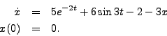
1. Consider
   • 
   1. Determine the analytical solution.
   2. Determine approximate numerical solutions using the first, second and third order Taylor series expansions for x(t+dt). You may write one computer program that computes all three of these or separate programs.
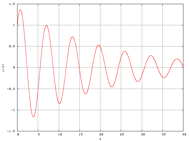
   3. On the same plot, graph the exact solution and three approximate solutions for a time step size of 0.5.
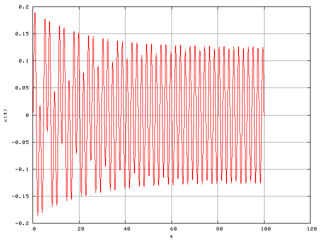
   4. On the same plot, graph the exact solution and three approximate solutions for a time step size of 0.25. For the three approximate solutions, did the ovarall average error decrease in the manner expected? By what factor did it decrease in each case?
   5. Comparing the value of the approximate solutions and the exact solutions after the very first step for the two different time steps, did the truncation error decrease as expected? By what factor did it decrease in each case?
2. Optional (50 points extra credit): use a Taylor series expansion to fouth order to determine an approximate numerical solution to the above equation. Also complete the error analysis.
3. The free response of a second order system is illustrated in the following figure. Determine the natural frequency and the damping ratio.
   • 
4. The following is a plot of the response of the system from the previous problem to the forcing function f(t)=cos(3t). Using this graph and the graph from the previous problem, can you find the mass, spring constant and damper constant? If so, what are they?
   • 

[tshinnic]

The first question asks for the analytical solution. What is that?

[goodwine]

The first question asks for the analytical solution. What is that?

http://www.everything2.com/index.pl?node_id=1457086

[goodwine]

The step sizes I specified for this problem won't work in a way that is intuitively obvious to you. What should happen if you use the step sizes indicated is the following:

1. The different order methods will work such that the third order method is better than the second order method, which in turn is better than the first order method in terms of the overall accuracy.
2. If you decrease the step size, the overall accuracy will improve to the degree that it should
3. However, the local truncation error will not behave as expected when you analyze the error after the first time step.
   1. Cutting the step size in half will not decrease the error after the first time step in the way you expect.
   2. Also, the third order methos is worse (after one time step) than the other methods.

The reason for this can be determined by considering the coefficients of the various powers of dt in the expansion. If you evaluate them at t=0, you will see that they vary by approximately an order of magnitude, so, in fact the time step has to be smaller than I indicated for the local truncation error analysis to behave the way you would expect.

If you make the time steps 10 times smaller, i.e., dt=0.05 and dt=0.025 things should behave properly.

I'll give 40 points extra credit if you modify your program to print the coefficients of the various powers of dt at each time step and then go back to your calculus book to find the equation for the magnitude of the remainder in a Taylor series and use that to determine exactly the point at which the local truncation error will behave properly.

The overall lesson here is that the rules for the errors only work for dt "small enough." Often this will simply be dt<1; however, if the problem is sufficiently weird (in this case the coefficients for the different dt terms in the Taylor series expansion were of different orders of magnitude), then it may require dt<<1.

[mattstorey]

problem 1 asks for the overall error, I know what it should be, but how do we go about finding it for our particular data

[goodwine]

problem 1 asks for the overall error, I know what it should be, but how do we go about finding it for our particular data

One way is just by looking at the plots. If the step size you used is too small, another option is, since you know the exact answer, to print the error at each time step for each of the methods to a file and then plot that. Then if you decrease the step size and replot the errors, they should decrease appropriately.

[mattstorey]

Im having some difficulty with problem 4, how does the addition of the forcing function make the problem different to solve than problem 3. should the homogeneous be found the same way and then determined before it decays?

[goodwine]

Im having some difficulty with problem 4, how does the addition of the forcing function make the problem different to solve than problem 3. should the homogeneous be found the same way and then determined before it decays?

Problem three gives you enough information to find the natural frequency and the damping ratio, but not m, b and k. There is enough additional information in the last problem to be able to use the results form the previous problem to find all three parameters.

[goodwine]

It didn't literally say it (it does now because I changed it), but I intended problem 4 to be based on problem 3. So you are to assume that the plot in problem 4 is the forced solution to the same system as in problem 3. Mathematically, you may use your answers from problem 3 to do what is needed in problem 4.