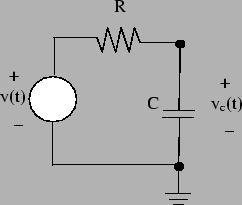
The first part of the circuit in figure
4 consists of a resistor, ![]() , and
capacitor,
, and
capacitor, ![]() connected in series. The circuit is shown
in figure 5. The circuit is driven by
a time-varying voltage
connected in series. The circuit is shown
in figure 5. The circuit is driven by
a time-varying voltage ![]() and we're interested in the
voltage
and we're interested in the
voltage ![]() that develops over the capacitor.
that develops over the capacitor.
We now assume that ![]() is a
is a ![]() -periodic pwm signal.
Over a
single period,
-periodic pwm signal.
Over a
single period, ![]() , the input voltage to the circuit
has two distinct parts. There is the "forced" part from
, the input voltage to the circuit
has two distinct parts. There is the "forced" part from
![]() during which the applied voltage is
during which the applied voltage is ![]() . In this
interval, the capacitor is being charged by the external
voltage source. After this charging phase, the applied
voltage drops to zero and the capacitor is discharging through its resistor.
. In this
interval, the capacitor is being charged by the external
voltage source. After this charging phase, the applied
voltage drops to zero and the capacitor is discharging through its resistor.
During the "charging" phase, we can think of the RC circuit
as being driven by a step function of magnitude ![]() volts.
If we assume that the capacitor has an initial voltage of
volts.
If we assume that the capacitor has an initial voltage of
![]() at time
at time ![]() (the start of the period), then the
circuit's response is simply the total response of the
system. So the capacitor's voltage is given by the
equation
(the start of the period), then the
circuit's response is simply the total response of the
system. So the capacitor's voltage is given by the
equation
During the "discharge" phase, there is no external voltage
being applied to the RC circuit. This means that the
system response is due solely to the capacitor voltage that
was present at time ![]() . As a result the capacitor's
voltage over the time interval
. As a result the capacitor's
voltage over the time interval ![]() is captured by the
RC circuit's natural response. So the capacitor's voltage
is given by the equation
is captured by the
RC circuit's natural response. So the capacitor's voltage
is given by the equation
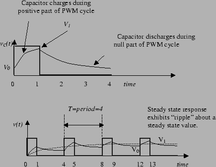
The top drawing in figure
6 illustrates the output signal
we expect from a PWM driven RC circuit over an interval
from ![]() . For times
. For times ![]() beyond this interval, we
expect to see the waveform shown in the bottom drawing in
figure 6. In this drawing we
assume that the capacitor is initially uncharged. As our
circuit cycles through its charge and discharge phases, the
voltage over the capacitor follows a saw-tooth trajectory
that eventually reaches a steady state regime. In this
steady-state region, the capacitor on the voltage zigzags
between
beyond this interval, we
expect to see the waveform shown in the bottom drawing in
figure 6. In this drawing we
assume that the capacitor is initially uncharged. As our
circuit cycles through its charge and discharge phases, the
voltage over the capacitor follows a saw-tooth trajectory
that eventually reaches a steady state regime. In this
steady-state region, the capacitor on the voltage zigzags
between ![]() and
and ![]() volts. The exact value of these
steady state voltages is dependent on the period
volts. The exact value of these
steady state voltages is dependent on the period ![]() and
the duty cycle
and
the duty cycle ![]() . What we now want to do is
characterize these voltages in terms of
. What we now want to do is
characterize these voltages in terms of ![]() and
and ![]() .
.
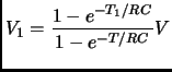
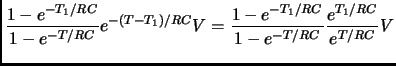
To determine ![]() and
and ![]() at steady state, we note that
at steady state, we note that
![]() is the capacitor's charge after the discharge phase.
Since we expect the steady state behavior to be
is the capacitor's charge after the discharge phase.
Since we expect the steady state behavior to be
![]() -periodic, we can conclude that
-periodic, we can conclude that
![]() which means that
which means that
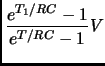
Equations 4 and 5 are
two nonlinear equations in to unknowns. We now try to
solve these equations. To start we insert equation
4 into equation 5 to
obtain
We now take equation 7 and back
substitute it into equation 4 to obtain
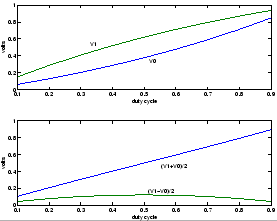
Figure 7 shows two graphs
characterizing the voltage, ![]() , over the capacitor as
a function of the duty cycle. In particular, these
graphs assume that
, over the capacitor as
a function of the duty cycle. In particular, these
graphs assume that ![]() volt,
volt, ![]() k-ohm,
k-ohm, ![]()
![]() F, and
the period
F, and
the period ![]() milliseconds. We've plotted duty
cycles at
milliseconds. We've plotted duty
cycles at ![]() to
to ![]() in increments of
in increments of ![]() . The top
graph plots
. The top
graph plots ![]() and
and ![]() . Note that these two values
have a symmetry around a steady state value. The steady
state value is simply the average of
. Note that these two values
have a symmetry around a steady state value. The steady
state value is simply the average of ![]() and
and ![]() .
We've plotted this value
.
We've plotted this value
![]() in the
second graph. We've also plotted the ripple
in the
second graph. We've also plotted the ripple
![]() in this graph. The important
thing to note here is that the average value of the
capacitor voltage varies in a linear manner with
duty cycle.
in this graph. The important
thing to note here is that the average value of the
capacitor voltage varies in a linear manner with
duty cycle.
Note that the ripple shown in figure
7 is about ![]() volts. Is it
possible to reduce this. Intuitively we might suppose
that if the period
volts. Is it
possible to reduce this. Intuitively we might suppose
that if the period ![]() is much smaller, then there is
less time to discharge to cap and this might result in a
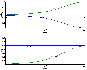
smaller ripple. To test this hypothesis, we plot the
ripple as a function of PWM period,
is much smaller, then there is
less time to discharge to cap and this might result in a
smaller ripple. To test this hypothesis, we plot the
ripple as a function of PWM period, ![]() . In this case,
we assume that
. In this case,
we assume that ![]() k-ohm,
k-ohm, ![]()
![]() F,
F, ![]() volt, and we fix the duty cycle at 50 percent. The
plots are shown in figure 8.
In these plots,
volt, and we fix the duty cycle at 50 percent. The
plots are shown in figure 8.
In these plots, ![]() ranges over two decades from
ranges over two decades from ![]() milliseconds to
milliseconds to ![]() milliseconds. What should be
apparent here is that as we decrease the period beneath
milliseconds. What should be
apparent here is that as we decrease the period beneath
![]() milliseconds that the ripple in our voltage
becomes negligible. This time, of course, is comparable
to the RC time constant of
milliseconds that the ripple in our voltage
becomes negligible. This time, of course, is comparable
to the RC time constant of ![]() seconds for this
circuit, which is entirely reasonable.
seconds for this
circuit, which is entirely reasonable.
What should be apparent from the preceding discussion
that the RC circuit essentially turns the pwm input
signal, ![]() , into a constant analog voltage with a
small ripple on it. We can make this ripple arbitrarily
small through proper selection of the period. Moreover,
we can see that the value of
, into a constant analog voltage with a
small ripple on it. We can make this ripple arbitrarily
small through proper selection of the period. Moreover,
we can see that the value of ![]() is proportional to
the pwm's duty cycle.
is proportional to
the pwm's duty cycle.
As we'll see below, it is relatively easy for the MicroStamp11 to generate a pwm signal through the use of output compare interrupts. This means that with the help of the RC circuit in figure 5, we can use the MicroStamp11 to generate an analog voltage that lies between zero and 5 volts. Moreover, we can tune this output voltage by simply tuning the duty cycle of the pwm signal. Unfortunately, there is one small problem with the circuit shown in figure 5. This problem and its solution are discussed in the next subsection.